UMAP flow and growth

Prepare celltype, time and barcode with ct.prepare_anndata before training or plotting; see input conventions. AnnData copies preserve source fields and order, and arrays can be assembled automatically.

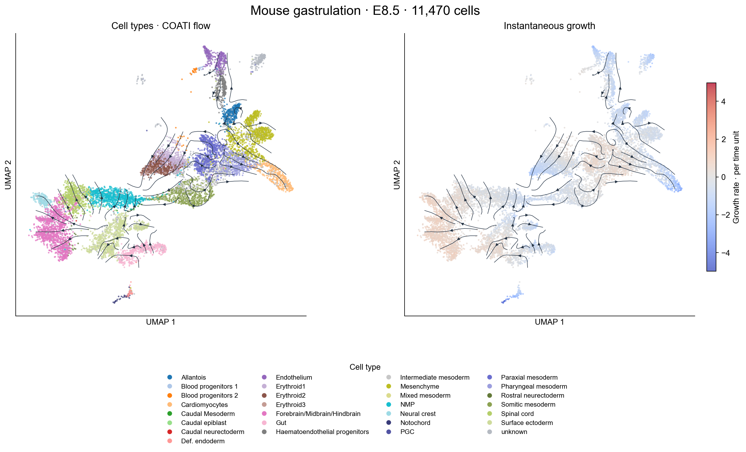
Cell types, growth and flow together

cells = ct.prepare_anndata(adata, use_rep="X_pca", time_key="day", celltype_key="cell_type")
result = ct.train_vector_field(cells, balanced=False)
axes = result.plot_dynamics(cells)
axes[0].figure.savefig("dynamics_umap.pdf", bbox_inches="tight")

# A growth heat map alone, or with streams:
result.plot_growth(cells)
result.plot_growth(cells, show_velocity=True)

# Explicitly store results on a copy:
stored = result.write_dynamics(cells, copy=True)
stored.obs["coati_growth"]
stored.obsm["coati_velocity_umap"]

An unbalanced model has two panels; a balanced model has a motion panel and no constructed growth values. Supplied cell-type labels are displayed at observed points near each group’s median. Existing Scanpy celltype_colors are reused; palette={"type_a": "#0072ce", "type_b": "#f28c28"} can override them. Both panels share the UMAP coordinates, cell order, axes limits and projected vectors.

The heat map displays instantaneous d log(weight)/dt, evaluated using the original training features and each cell’s observation time. It follows the saved ODE exactly, including its alpha_growth multiplier. It is different from cumulative log_weights, total population mass, or an experimental proliferation measurement. Positive rates increase mass; negative rates reduce it.

growth = result.compute_growth()
growth = result.compute_growth(cells.obsm["X_pca"], time=cells.obs["time"].to_numpy())
# Subset a stage to avoid mixing different observation-time fields:
result.plot_dynamics(cells[cells.obs["time"] == 1.].copy())

time=.5 evaluates a field at one common time on the displayed coordinates; it does not transport those cells to that time. Growth is unavailable for balanced models. The image and biological tutorial use a 1,000-iteration multimodal unbalanced gastrulation run on all four observed stages. The plot shows all 11,470 E8.5 cells at their shared model time t = 2, with supplied cell-type names in the legend. RNA50 and paired ATAC14 inputs are already scaled; the source RNA UMAP is reused. Source data: Argelaguet and colleagues, GSE205117, with prepared inputs from TraInfBench. This is a short workflow demonstration, not a convergence or proliferation claim.

Run examples/run_gastrulation_dynamics.py --data-dir /path/to/gastrulation --output outputs/gastrulation-dynamics --iterations 1000 to reproduce the example. The toy script examples/run_dynamics.py remains available for a small input check.

Existing velocity interface

A trained COATI model exposes its primary-space velocity field without integrating trajectories. It supports single- or multi-modal training, and balanced or unbalanced dynamics. The result can be reloaded and used for the same analyses.

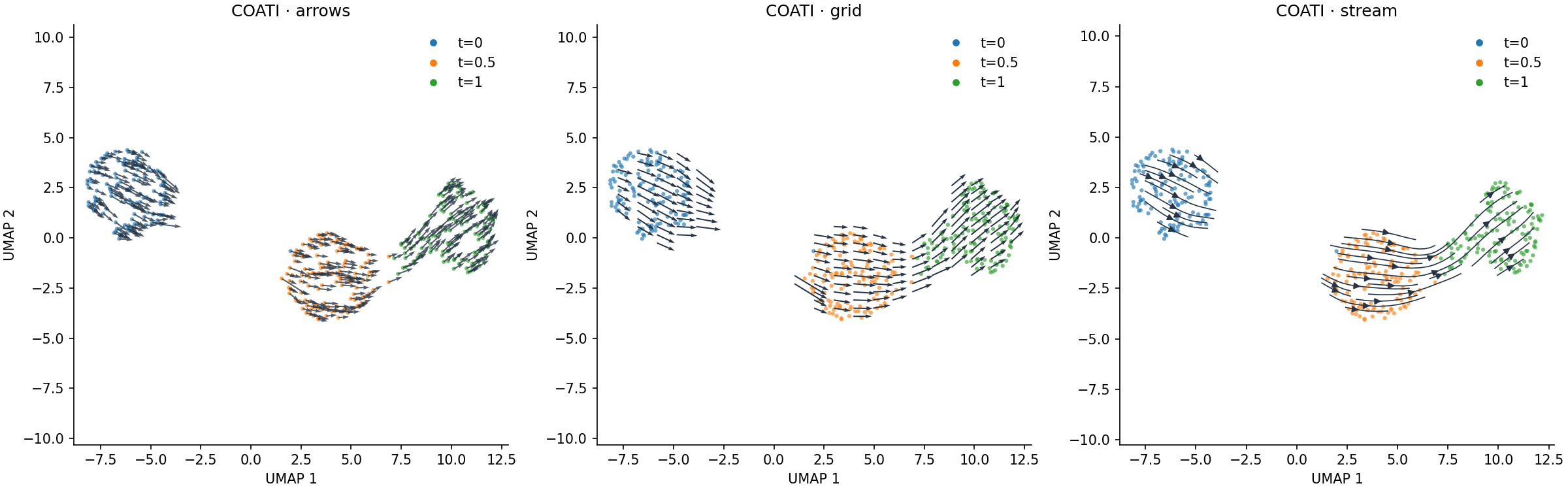
This figure uses a short synthetic multimodal unbalanced run and an actual fitted UMAP.

Evaluate the field

v = result.compute_velocity()  # snapshot rows concatenated in data order
v = result.compute_velocity(adata.obsm["X_pca"], time=adata.obs["time"].to_numpy())
v_at_half = result.compute_velocity(adata.obsm["X_pca"], time=.5)
trajectory = result.predict_trajectory()  # integration is a separate operation

Input features, feature order and preprocessing must match the model. With raw=True (the default), points and velocities use input units, including reversal of an explicit training normalization scale. Velocity is displacement per unit of the numeric training time. Unbalanced velocities are spatial motion; growth rates are not included in arrows.

Plot AnnData without modifying it

result.plot_velocity(adata, use_rep="X_pca", time_key="time", color="cell_type", style="stream")
result.plot_velocity(adata, use_rep="X_pca", time_key="time", color="time", style="grid")
result.plot_velocity(adata, use_rep="X_pca", time_key="time", style="arrows")

Use use_rep=None if the model was trained directly on adata.X. basis=”umap” reads adata.obsm[“X_umap”]; basis=”tsne” reads X_tsne. Existing coordinates are required. The function neither fits an embedding nor changes AnnData. All calculations use AnnData’s current row order, so subsets and reordered cells remain aligned.

For categorical stages, map them to the same numeric times used in training:

result.plot_velocity(adata, use_rep="X_pca", time_key="stage",
                     time_mapping={"early":0., "middle":.5, "late":1.},
                     color="cell_type")

Without a time override, each cell uses its own observation time. A combined plot summarizes time-dependent vectors and smooths neighboring values for display; it is not a field at one common time. For a common-time view pass time=.5. For a stage-specific view pass an AnnData subset from that stage.

Projection and smoothing

The model is evaluated in the representation where it was trained. For each cell, neighboring displacements in this representation and corresponding embedding displacements define a regularized local linear map. That map sends the learned velocity into the existing 2D coordinates. This is an estimated local projection, not the analytic derivative of UMAP, and does not reproduce scVelo’s transition probability algorithm. UMAP distortions can change apparent direction and speed.

n_neighbors (30 by default) and ridge (1e-3) control this projection. Stream/grid plots then smooth projected vectors in embedding space; smooth, grid_size and min_mass control the display. Unsupported grid regions are masked using local sampling support and the observed convex hull. This avoids drawing streams across large empty regions between disconnected populations. Arrows are automatically scaled for display; numerical projected vectors retain their original magnitude.

These plots use the cell-arrow, grid-arrow and streamline forms described in the scVelo plotting documentation. The vectors come from COATI’s fitted vector field, rather than splicing kinetics.

Save vectors or use NumPy

field = result.compute_velocity_embedding(adata, use_rep="X_pca", time_key="time")
field.coordinates  # cells × 2
field.velocity     # cells × 2; numeric vectors, without display autoscaling

# Explicitly modify AnnData, or request a copy.
with_velocity = result.write_velocity(adata, copy=True, use_rep="X_pca", time_key="time")
with_velocity.obsm["coati_velocity"]
with_velocity.obsm["coati_velocity_umap"]

# Arrays in corresponding row order are also supported.
result.plot_velocity(embedding=umap_coordinates, points=primary_coordinates,
                     time=cell_times, color=cell_types, style="stream")

write_velocity defaults to modifying the supplied AnnData and returns it; copy=True leaves the input unchanged. This is the only plotting workflow that writes vectors. For CLI plotting, use coati plot-velocity --help. For a fully runnable toy example, use examples/run_velocity.py for the plotting API, the synthetic data experiments for a controlled toy, or gastrulation dynamics for biological AnnData.