Unbalanced Gaussian bump

Repeat the Gaussian-bump comparison with population growth. The data and frozen map are identical to the balanced tutorial. The terminal population mass is explicitly set to twice the initial mass. Compare beta = 1 and beta = 0.1, with and without synchronization, and show instantaneous growth along every learned trajectory.

from pathlib import Path
import sys
import uuid

example_dir = next(parent / "examples" for parent in (Path.cwd(), *Path.cwd().parents)
                   if (parent / "examples" / "synthetic" / "gaussian_assets.py").is_file())
if str(example_dir) not in sys.path:
    sys.path.insert(0, str(example_dir))

import anndata as ad
import numpy as np
import pandas as pd
import torch
import matplotlib.pyplot as plt
import coati as ct
from synthetic.gaussian_map import evaluate_bump_map, plot_map_performance
from synthetic.gaussian_comparison import (
    make_shared_initial_checkpoint,
    plot_gaussian_sync,
    plot_bump_height,
    compare_gaussian_runs,
)
from synthetic.gaussian_assets import load_shared_gaussian_assets, resolve_asset_directory

%matplotlib inline
torch.set_num_threads(1)
plt.rcParams.update({"font.family": "Arial", "font.size": 11})
run_dir = Path("outputs") / ("gaussian-bump-" + uuid.uuid4().hex[:8])
run_dir.mkdir(parents=True)
print("Result directory:", run_dir)

from synthetic.gaussian_assets import plot_growth_along_trajectories

Result directory: outputs/gaussian-bump-89dd1efe

Shared data and map

The observed snapshots contain 1,000 initial and 2,000 terminal cells. Reusing the same assets isolates the effect of unbalanced training rather than changing the geometry.

asset_dir = resolve_asset_directory()
cells, T, map_payload = load_shared_gaussian_assets(directory=asset_dir)
map_pairs = ad.read_h5ad(asset_dir / "map_pairs.h5ad")
data = ct.TemporalData.from_anndata(
    cells, obsm_key="X_latent", secondary_obsm_key="X_secondary"
)

summary = cells.obs.groupby(["time", "celltype"], observed=True).size().rename("Cells").to_frame()
assert [len(snapshot) for snapshot in data.primary] == [1000, 2000]
assert not any(parameter.requires_grad for parameter in T.parameters())
summary

		Cells
time	celltype
0.0	Initial	1000
1.0	Terminal A	1000
	Terminal B	1000

Inspect the frozen map

map_scores, map_grid = evaluate_bump_map(T, map_pairs, grid_n=96)
display(map_scores.round(6))
plot_map_performance(map_grid)
plt.show()
print(f"Best validation step: {map_payload['fit']['best_step']}")
print(f"Grid z correlation: {map_grid['z_correlation']:.6f}")
print(f"Learned height at (0.5, 0.5): {map_grid['center_predicted_height']:.6f}")

	Pairs	XY_RMSE	Z_RMSE	Z_MAE
Evaluation
Held-out observed	434	0.000047	0.021079	0.004067
Held-out support	1066	0.000065	0.005544	0.003500
Independent grid	9216	0.000067	0.005036	0.002998

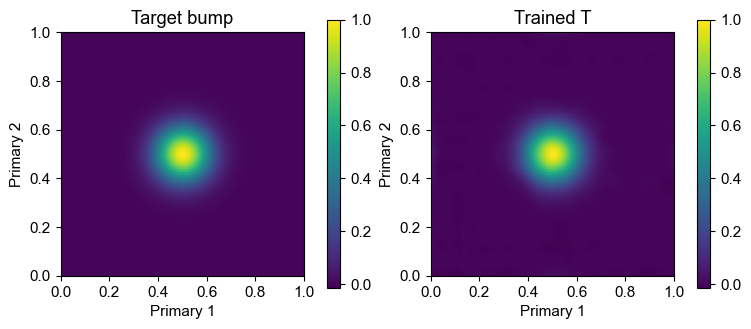
Best validation step: 1500
Grid z correlation: 0.999378
Learned height at (0.5, 0.5): 0.999919

Configure unbalanced transport

balanced=False enables the growth field and mass-matching loss. biological_num=[1, 2] is the relative population-mass prior, so the target terminal mass is 2. The observed sample counts imply the same ratio, but writing the prior explicitly makes the intended experiment independent of future resampling. mass_weight=100 and global_mass=True enforce both local allocation and total population mass. In the implementation, beta is growth_weight, the alpha_growth coefficient multiplying the learned growth rate and growth action.

base_config = ct.Config(
    multimodal=True,
    balanced=False,
    iterations=3000,
    batch_size=256,
    hidden_dim=256,
    secondary_weight=.5,
    growth_weight=1.,
    mass_weight=100.,
    global_mass=True,
    extra={
        "biological_num": [1.0, 2.0],
        "median_n_sample": 512,
        "floor_n_sample": 256,
        "adaptive_lambda": True,
    },
)
configs = {}
for beta in [1.0, .1]:
    beta_config = base_config.with_parameters(growth_weight=beta)
    configs[f"beta={beta:g} | Without sync"] = beta_config.with_parameters(
        multimodal=False, secondary_weight=0.
    )
    configs[f"beta={beta:g} | With sync"] = beta_config

pd.DataFrame({name: {key: cfg.to_dict()[key] for key in
    ["niters", "num_samples", "sync_loss", "sync_weight", "unbalancedModel",
     "alpha_growth", "mass_loss", "mass_coefficient", "global_mass", "biological_num"]}
    for name, cfg in configs.items()})

	beta=1 | Without sync	beta=1 | With sync	beta=0.1 | Without sync	beta=0.1 | With sync
niters	3000	3000	3000	3000
num_samples	256	256	256	256
sync_loss	False	True	False	True
sync_weight	0.0	0.5	0.0	0.5
unbalancedModel	True	True	True	True
alpha_growth	1.0	1.0	0.1	0.1
mass_loss	True	True	True	True
mass_coefficient	100.0	100.0	100.0	100.0
global_mass	True	True	True	True
biological_num	[1.0, 2.0]	[1.0, 2.0]	[1.0, 2.0]	[1.0, 2.0]

Train the vector and growth fields

All four runs start from identical unbalanced network weights. Each model contains a velocity field and an instantaneous log-growth field; only beta and synchronization differ.

initial = make_shared_initial_checkpoint(base_config, run_dir / "initial.pt")
results = {}
for name, cfg in configs.items():
    print("Training:", name, flush=True)
    slug = name.lower().replace(" | ", "-").replace("=", "").replace(".", "p").replace(" ", "-")
    results[name] = ct.train_vector_field(
        cells, cfg, use_rep="X_latent", secondary_obsm_key="X_secondary",
        T_model=T if cfg.multimodal else None,
        output_dir=run_dir / slug,
        warm_start_path=initial,
    )

Training: beta=1 | Without sync

Training: beta=1 | With sync

Training: beta=0.1 | Without sync

Training: beta=0.1 | With sync

Learned trajectories

predictions = {}
for name, result in results.items():
    prediction = result.predict_trajectory(times=np.linspace(0., 1., 51), method="rk4")
    with torch.no_grad():
        prediction["secondary"] = T(torch.as_tensor(prediction["primary"], dtype=torch.float32)).numpy()
    predictions[name] = prediction

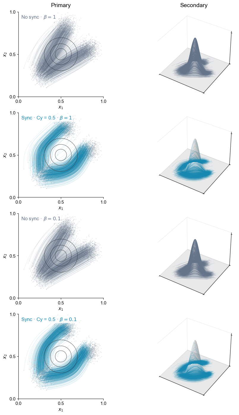
plot_gaussian_sync(data, T, results, predictions)
plt.show()
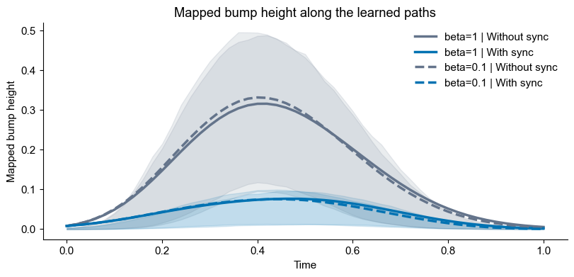
plot_bump_height(predictions)
plt.show()

Growth along trajectories

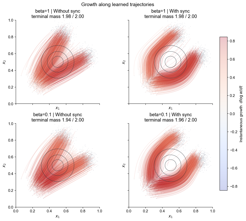
Blue segments indicate negative instantaneous growth and red segments indicate positive instantaneous growth. The colour is the fitted \(d\log w/dt\) evaluated along each path; the title reports the integrated terminal mass against the target of 2. Because both terminal populations expand in this example, the learned raw growth may remain positive and therefore use mainly the red half of the diverging scale.

growth_figure, growth = plot_growth_along_trajectories(data, results, predictions)
plt.show()

Mass and transport diagnostics

scores = compare_gaussian_runs(results, predictions)
display(scores.T.round(6))
pd.DataFrame({name: result.evaluate() for name, result in results.items()}).T.round(6)

Model	beta=1 | Without sync	beta=1 | With sync	beta=0.1 | Without sync	beta=0.1 | With sync
Primary endpoint Sinkhorn	0.000653	0.001105	0.000491	0.000484
Primary kinetic energy	0.200886	0.241582	0.209753	0.260358
Secondary kinetic energy	1.372201	0.322865	1.362476	0.328599
Predicted terminal mass	1.980399	1.981807	1.940608	1.962171
Target terminal mass	2.000000	2.000000	2.000000	2.000000
Median maximum bump height	0.380701	0.043216	0.380506	0.045225
States outside unit square	0.000000	0.000000	0.000000	0.000000

	endpoint_sinkhorn_before	endpoint_sinkhorn_after	kinetic_energy_mean	endpoint_sampling_floor	predicted_mass_ratio	observed_count_ratio	secondary_endpoint_sinkhorn
beta=1 | Without sync	0.165117	0.000780	0.000201	0.000348	1.980400	2.0	NaN
beta=1 | With sync	0.165117	0.000917	0.000242	0.000348	1.981807	2.0	0.000928
beta=0.1 | Without sync	0.165117	0.000521	0.000210	0.000348	1.940608	2.0	NaN
beta=0.1 | With sync	0.165117	0.000482	0.000260	0.000348	1.962171	2.0	0.000488