Held-out biological reconstruction

Remove E15.5 from the paired pancreas snapshots, train on E14.5 and E16.5 for 1,000 vector-field iterations, and reconstruct the missing distribution at its original time.

Both the FiLM map T and the vector field use only the retained stages. This notebook uses the existing, frozen RNA PCA50 / ATAC PoissonVI22 representations, with optional scalar normalization; it is a temporal holdout in that representation, rather than an end-to-end raw-data holdout. Balanced mode compares probability distributions, not absolute cell counts.

Install the notebook and visualization extras with python -m pip install -e '.[notebooks,visualization]'. The paired reduced inputs are available in TraInfBench. Set COATI_BIO_DATA to their directory if TraInfBench is not a sibling checkout.

from pathlib import Path
from datetime import datetime, timezone
import os
import hashlib
import json
import time

import anndata as ad
import numpy as np
import pandas as pd
import matplotlib.pyplot as plt
import torch
from geomloss import SamplesLoss
from IPython.display import display
from umap import UMAP
import coati as ct

%matplotlib inline

SEED = 0
root = next(p for p in (Path.cwd(), *Path.cwd().parents)
            if (p / "pyproject.toml").exists() and (p / "src/coati").is_dir())
data_dir = Path(os.environ.get("COATI_BIO_DATA", root.parent / "TraInfBench/data/processed/pancreas"))
run_dir = root / "outputs" / ("pancreas-heldout-1000-" + datetime.now(timezone.utc).strftime("%Y%m%dT%H%M%S%fZ"))
plt.rcParams.update({"font.family": "Arial", "font.size": 11, "axes.spines.top": False,
                     "axes.spines.right": False, "figure.dpi": 120})

Load paired AnnData

Keep RNA and ATAC rows paired. X_latent contains the prepared, normalized model inputs; X_reduced_raw contains the same reduced features before scalar normalization. Neither representation contains raw gene expression or peak counts. The source dataset is GSE275562, with processed inputs prepared through the moscot workflow.

rna = ad.read_h5ad(data_dir / "rna.h5ad")
atac = ad.read_h5ad(data_dir / "atac.h5ad")
assert rna.obs_names.equals(atac.obs_names), "RNA and ATAC cell identities must match."
assert np.array_equal(rna.obs["stage"].to_numpy(), atac.obs["stage"].to_numpy())
assert np.array_equal(rna.obs["time_point_processed"].to_numpy(), atac.obs["time_point_processed"].to_numpy())

stages = ["E14.5", "E15.5", "E16.5"]
times = np.array([0., 1., 2.])
heldout_time = 1.
heldout_stage = "E15.5"
row_times = rna.obs["time_point_processed"].to_numpy(dtype=float)
for stage, t in zip(stages, times):
    assert np.all(row_times[rna.obs["stage"].to_numpy() == stage] == t)

training_rows = row_times != heldout_time
training_times = times[times != heldout_time]
assert training_times.tolist() == [0., 2.]

display(pd.DataFrame({"Stage": stages, "Time": times,
                      "Cells": [int((row_times == t).sum()) for t in times],
                      "Use": ["Train", "Held out", "Train"]}))
print("RNA dimensions:", rna.obsm["X_latent"].shape[1])
print("ATAC dimensions:", atac.obsm["X_latent"].shape[1])

	Stage	Time	Cells	Use
0	E14.5	0.0	9029	Train
1	E15.5	1.0	10333	Held out
2	E16.5	2.0	3242	Train

RNA dimensions: 50
ATAC dimensions: 22

Optional normalization

Set normalize = True to estimate one W2-based scalar per modality from X_reduced_raw. With False (the default), reuse X_latent without further scaling.

Only the retained snapshots determine the scales. Apply each fixed scale to all observations in that modality, including the held-out reference. A scalar preserves the relative sizes of the reduced coordinates; it does not standardize every feature separately.

\[ s_m^2 = \sum_i \frac{D^{(2)}_{\varepsilon_{\mathrm{norm}}}(\rho^{(m)}_{t_i},\rho^{(m)}_{t_{i+1}})}{t_{i+1}-t_i},\qquad z^{(m)} = x^{(m)}/s_m. \]

Here \(D^{(2)}\) is the debiased Sinkhorn approximation with cost \(\frac12\lVert x-y\rVert^2\). The scales use 512 sampled cells per retained snapshot, a fixed seed and a small normalization regularization \(\varepsilon_{\mathrm{norm}}=10^{-8}\). This is an estimate of the W2 scale, not an exact full-data OT solve. The original PCA/PoissonVI representations remain fixed.

normalize = False
input_representation = "X_reduced_raw" if normalize else "X_latent"
model_features = {
    "RNA": np.asarray(rna.obsm[input_representation], dtype=np.float32).copy(),
    "ATAC": np.asarray(atac.obsm[input_representation], dtype=np.float32).copy(),
}
normalization_scales = {"RNA": 1., "ATAC": 1.}

if normalize:
    normalization_epsilon = 1e-8
    normalization_samples = 512
    scale_rng = np.random.default_rng(SEED)
    scale_loss = SamplesLoss("sinkhorn", p=2, blur=np.sqrt(normalization_epsilon),
                             debias=True, backend="tensorized")
    with torch.no_grad():
        for modality, features in model_features.items():
            retained = []
            for t in training_times:
                snapshot = features[row_times == t]
                rows = scale_rng.choice(len(snapshot), size=min(normalization_samples, len(snapshot)), replace=False)
                retained.append(torch.tensor(snapshot[rows]))
            action = sum(float(scale_loss(x, y)) / (t1 - t0)
                         for x, y, t0, t1 in zip(retained[:-1], retained[1:],
                                               training_times[:-1], training_times[1:]))
            if not np.isfinite(action) or action <= 0:
                raise ValueError(f"Cannot estimate a positive W2 scale for {modality}.")
            normalization_scales[modality] = float(np.sqrt(action))
            model_features[modality] = features / normalization_scales[modality]

# Build private working inputs without modifying either source AnnData file.
paired = rna.copy()
paired.obsm["X_latent"] = model_features["RNA"]
paired.obsm["X_atac"] = model_features["ATAC"]
observed = ct.TemporalData.from_anndata(
    paired, time_key="stage", obsm_key="X_latent", secondary_obsm_key="X_atac",
    time_order=stages, times=times,
)
training = observed.without_times([heldout_time])
assert training.times.tolist() == [0., 2.]
assert training.labels == ["E14.5", "E16.5"]
display(pd.DataFrame({"Modality": ["RNA", "ATAC"],
                      "Input representation": input_representation,
                      "Normalize": normalize,
                      "Scalar": list(normalization_scales.values())}))

	Modality	Input representation	Normalize	Scalar
0	RNA	X_latent	False	1.0
1	ATAC	X_latent	False	1.0

Train on the two retained stages

The settings below are a short demonstration, chosen before inspecting the held-out result. Map pretraining uses at most 300 epochs with early stopping on validation cells from the retained stages. The vector field then trains for exactly 1,000 iterations. No checkpoint, loss, manifold reference or map-training pair contains E15.5.

config = ct.Config(
    multimodal=True, balanced=True, iterations=1000, batch_size=128,
    learning_rate=1e-3, hidden_dim=128, n_layers=2, dt=0.1,
    secondary_weight=0.35, matching_weight=50., energy_weight=1.,
    manifold_weight=0.1, sync_density_loss=True, seed=SEED, device="cpu",
)
map_config = ct.MapConfig(epochs=300, patience=30)
started = time.perf_counter()
result = ct.train_vector_field(training, config, map_config=map_config, output_dir=run_dir)
training_seconds = time.perf_counter() - started
checkpoint = torch.load(run_dir / "checkpoints/path_param.pth", map_location="cpu", weights_only=True)
assert checkpoint["iteration"] == 1000
assert result.data.times.tolist() == [0., 2.]
assert result.map_report["training_times"] == [0., 2.]
assert heldout_time not in result.map_report["training_times"]
print(f"Vector-field iterations: {checkpoint['iteration']}")
print(f"Training time (including map): {training_seconds:.1f} seconds")
print("T training stages:", result.map_report["training_labels"])
print("T validation status:", result.map_report["status"])
print("T best epoch:", result.map_report["best_epoch"])
print("Checkpoint:", run_dir / "checkpoints/path_param.pth")

Vector-field iterations: 1000
Training time (including map): 34.1 seconds
T training stages: ['E14.5', 'E16.5']
T validation status: passed
T best epoch: 35
Checkpoint: /Users/jingfeng/local/project/COATI/outputs/pancreas-heldout-1000-20261012T184239774396Z/checkpoints/path_param.pth

Query the missing time

Integrate from E14.5 on a 0.1-spaced grid and read the state at t = 1.0. The query does not turn that time into a training observation. A reproducible sample of 4,000 initial cells represents the inferred distribution; their original identities do not provide ground-truth correspondences to cells at E15.5.

rng = np.random.default_rng(SEED)
initial_rows = rng.choice(len(training.primary[0]), size=min(4000, len(training.primary[0])), replace=False)
query_times = np.linspace(0., 2., 21)
prediction = result.predict_trajectory(initial=training.primary[0][initial_rows], times=query_times, method="rk4")
secondary_prediction = result.project_secondary(prediction)
middle_index = int(np.flatnonzero(np.isclose(query_times, heldout_time))[0])
reconstructed = {"RNA": prediction["primary"][middle_index],
                 "ATAC": secondary_prediction[middle_index]}
heldout = {"RNA": observed.primary[1], "ATAC": observed.secondary[1]}
for modality in reconstructed:
    assert np.isfinite(reconstructed[modality]).all()
    print(modality, "held-out observation", heldout[modality].shape,
          "reconstruction", reconstructed[modality].shape)
np.savez_compressed(run_dir / "heldout_prediction.npz", times=query_times,
                    primary=prediction["primary"], secondary=secondary_prediction,
                    initial_rows=initial_rows)

# Verify that the saved model reproduces both modalities at the queried time.
restored = ct.load_result(run_dir)
check = restored.predict_trajectory(initial=training.primary[0][initial_rows[:32]], times=query_times)
np.testing.assert_allclose(check["primary"], prediction["primary"][:, :32], rtol=2e-5, atol=2e-6)
np.testing.assert_allclose(restored.project_secondary(check), secondary_prediction[:, :32], rtol=2e-5, atol=2e-6)
print("Checkpoint reload agrees with the reconstruction.")

# Convert the held-out prediction back to the selected input representation.
reconstructed_input_units = {modality: points * normalization_scales[modality]
                             for modality, points in reconstructed.items()}
np.savez_compressed(run_dir / "heldout_input_units.npz", **reconstructed_input_units)
_ = (run_dir / "normalization.json").write_text(json.dumps({
    "enabled": normalize, "input_representation": input_representation,
    "scales": normalization_scales, "fit_times": training_times.tolist() if normalize else [],
}, indent=2) + "\n")

RNA held-out observation (10333, 50) reconstruction (4000, 50)
ATAC held-out observation (10333, 22) reconstruction (4000, 22)

Checkpoint reload agrees with the reconstruction.

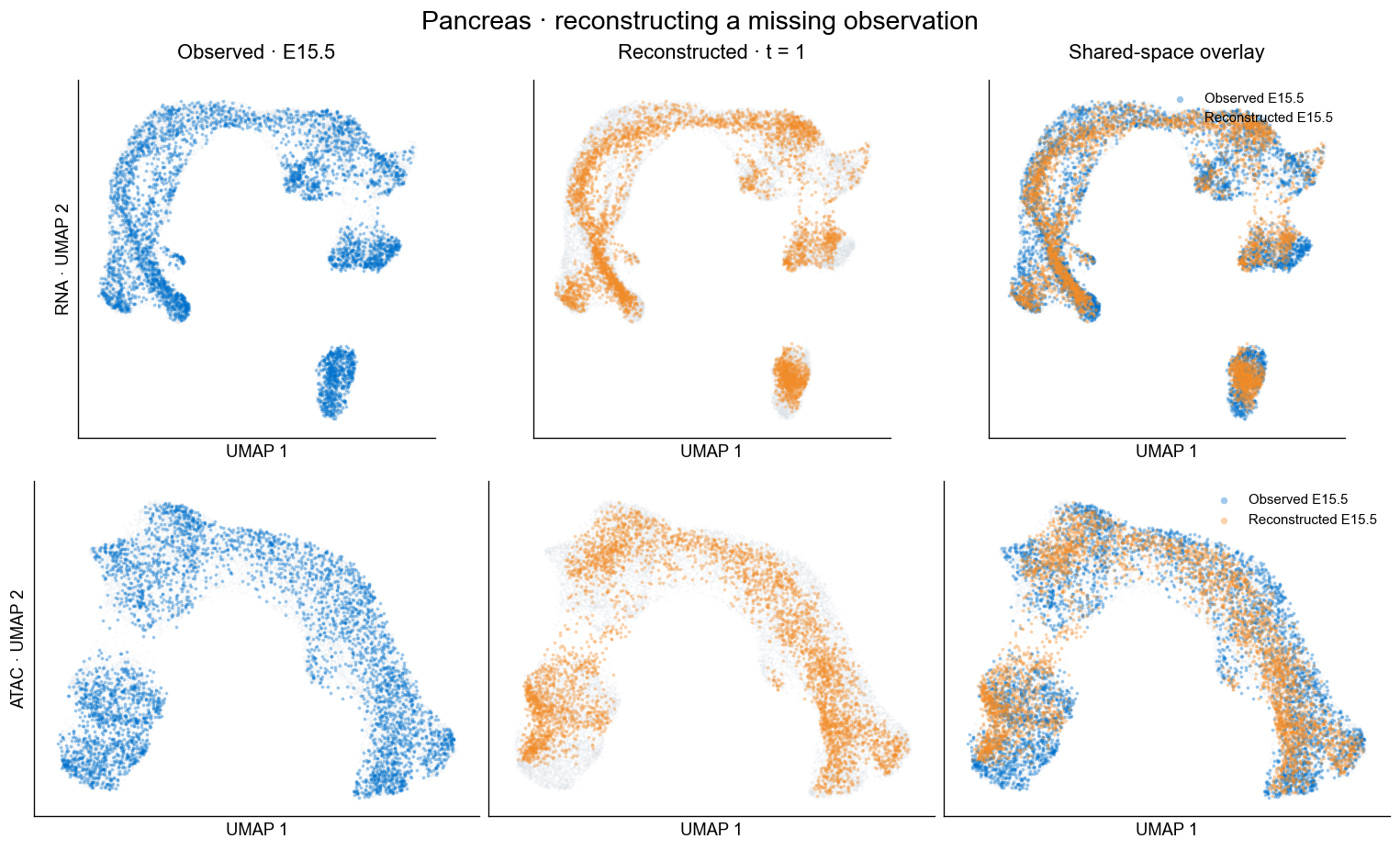
Put real and predicted cells in a shared UMAP

A coordinate array alone cannot project new points. Fit one UMAP per modality on the retained observations only, then freeze it and transform the held-out observations and predictions together. The same axes and projector are used in every panel. These are new display embeddings, not the stored source UMAPs. UMAP is for visualization; quantify reconstruction in the original normalized model space below.

display_coordinates = {}
projectors = {}
training_rows = row_times != heldout_time
for modality in ("RNA", "ATAC"):
    features = model_features[modality]
    projector = UMAP(n_neighbors=30, min_dist=0.35, n_components=2,
                     metric="euclidean", random_state=SEED, transform_seed=SEED,
                     n_jobs=1, n_epochs=300, low_memory=True)
    projector.fit(features[training_rows])
    observed_coordinates = projector.transform(features)
    predicted_coordinates = projector.transform(reconstructed[modality])
    projectors[modality] = projector
    display_coordinates[modality] = {
        "context": observed_coordinates,
        "observed": observed_coordinates[row_times == heldout_time],
        "predicted": predicted_coordinates,
    }
    print(modality, "shared UMAP ready")
np.savez_compressed(run_dir / "heldout_umap.npz", **{
    f"{modality.lower()}_{key}": values
    for modality, coordinates in display_coordinates.items()
    for key, values in coordinates.items()
})

RNA shared UMAP ready

ATAC shared UMAP ready

fig, axes = plt.subplots(2, 3, figsize=(12.6, 7.6), layout="constrained")
for row, modality in enumerate(("RNA", "ATAC")):
    coordinates = display_coordinates[modality]
    real = coordinates["observed"]
    predicted = coordinates["predicted"]
    plot_rng = np.random.default_rng(SEED)
    real = real[plot_rng.choice(len(real), size=min(4000, len(real)), replace=False)]
    combined = np.concatenate([coordinates["context"], predicted])
    low, high = combined.min(axis=0), combined.max(axis=0)
    pad = np.maximum((high - low) * 0.06, 0.1)
    for column, ax in enumerate(axes[row]):
        context = coordinates["context"]
        ax.scatter(context[:, 0], context[:, 1], s=2, c="#DDE3E8", alpha=0.2,
                   linewidths=0, rasterized=True)
        if column in (0, 2):
            ax.scatter(real[:, 0], real[:, 1], s=5, c="#0072CE", alpha=0.38,
                       linewidths=0, label="Observed E15.5", rasterized=True)
        if column in (1, 2):
            ax.scatter(predicted[:, 0], predicted[:, 1], s=5, c="#F28C28", alpha=0.38,
                       linewidths=0, label="Reconstructed E15.5", rasterized=True)
        ax.set(xlim=(low[0] - pad[0], high[0] + pad[0]), ylim=(low[1] - pad[1], high[1] + pad[1]),
               xlabel="UMAP 1", ylabel=f"{modality} · UMAP 2" if column == 0 else "")
        ax.set_aspect("equal", adjustable="box")
        ax.set_xticks([])
        ax.set_yticks([])
        if row == 0:
            ax.set_title(("Observed · E15.5", "Reconstructed · t = 1", "Shared-space overlay")[column], pad=14)
    axes[row, 2].legend(loc="upper right", frameon=False, markerscale=2, fontsize=9)
fig.suptitle("Pancreas · reconstructing a missing observation", fontsize=17)
fig.savefig(run_dir / "heldout_reconstruction_umap.png", dpi=200, bbox_inches="tight")
fig.savefig(run_dir / "heldout_reconstruction_umap.pdf", bbox_inches="tight")
plt.show()

Measure distribution reconstruction outside UMAP

Use debiased Sinkhorn divergence with \(p=2\) in the model representations. Lower is better. All comparisons use 512 points per distribution and five deterministic repeats. The empirical observed-split score is a sampling reference; the endpoint-mixture baseline puts equal probability on the two retained stages without learning dynamics. These comparisons evaluate probability distributions, not population growth.

The table reports the entropic regularization parameter \(\varepsilon\), with \(\varepsilon=(0.05\,\mathrm{median}\lVert x_i-x_j\rVert)^2\) in each held-out modality. For \(p=2\), GeomLoss takes its square root as the length-scale argument blur; the table uses \(\varepsilon\), as defined in the GeomLoss API. This evaluation setting does not alter the trained model.

metric_rows = []
for modality, snapshots in (("RNA", observed.primary), ("ATAC", observed.secondary)):
    target = torch.tensor(heldout[modality])
    predicted = torch.tensor(reconstructed[modality])
    metric_rng = np.random.default_rng(SEED + 10)
    median_rows = metric_rng.choice(len(target), size=512, replace=False)
    distances = torch.pdist(target[median_rows])
    regularization_scale = max(0.05 * float(distances.median()), 1e-6)
    epsilon = regularization_scale ** 2
    divergence = SamplesLoss("sinkhorn", p=2, blur=np.sqrt(epsilon), debias=True, backend="tensorized")
    scores = {"Reconstruction": [], "Initial distribution": [], "Endpoint mixture": [], "Observed split": []}
    with torch.no_grad():
        for repeat in range(5):
            target_rows = metric_rng.choice(len(target), size=1024, replace=False)
            reference = target[target_rows[:512]]
            independent = target[target_rows[512:]]
            prediction_rows = metric_rng.choice(len(predicted), size=512, replace=False)
            initial = torch.tensor(snapshots[0][metric_rng.choice(len(snapshots[0]), size=512, replace=False)])
            mixture = torch.tensor(np.concatenate([
                snapshots[0][metric_rng.choice(len(snapshots[0]), size=256, replace=False)],
                snapshots[-1][metric_rng.choice(len(snapshots[-1]), size=256, replace=False)],
            ]))
            for name, sample in (("Reconstruction", predicted[prediction_rows]),
                                 ("Initial distribution", initial), ("Endpoint mixture", mixture),
                                 ("Observed split", independent)):
                scores[name].append(float(divergence(sample, reference)))
    for name, values in scores.items():
        metric_rows.append({"Modality": modality, "Comparison": name,
                            "Mean": float(np.mean(values)), "SD": float(np.std(values, ddof=1)),
                            "Regularization ε": epsilon, "Points": 512, "Repeats": 5})
metrics = pd.DataFrame(metric_rows)
metrics.to_csv(run_dir / "heldout_metrics.csv", index=False)
display(metrics[["Modality", "Comparison", "Mean", "SD", "Regularization ε"]]
        .rename(columns={"Regularization ε": "ε"}).round(5))

	Modality	Comparison	Mean	SD	ε
0	RNA	Reconstruction	0.37956	0.00974	0.01488
1	RNA	Initial distribution	0.63991	0.03310	0.01488
2	RNA	Endpoint mixture	0.39044	0.01051	0.01488
3	RNA	Observed split	0.32654	0.00482	0.01488
4	ATAC	Reconstruction	0.49141	0.01736	0.02048
5	ATAC	Initial distribution	0.77943	0.04277	0.02048
6	ATAC	Endpoint mixture	0.45730	0.01704	0.02048
7	ATAC	Observed split	0.38675	0.01236	0.02048

Save the audit and inspect the result

The figures and scores are the outcome of this one short run, including any reconstruction error. No setting or checkpoint is selected using E15.5. A small UMAP separation is not proof of a good distribution match; use the representation-space scores as well. The existing all-data preprocessing remains fixed, so this experiment tests the exclusion of the middle stage from T and dynamics training, not exclusion from the original PCA/PoissonVI preprocessing.

audit = {
    "dataset": "pancreas", "seed": SEED, "heldout_stage": heldout_stage,
    "heldout_time": heldout_time, "training_stages": training.labels,
    "training_times": training.times.tolist(), "map_training_times": result.map_report["training_times"],
    "vector_field_iterations": checkpoint["iteration"], "training_seconds": training_seconds,
    "map_status": result.map_report["status"], "map_best_epoch": result.map_report["best_epoch"],
    "mode": "multimodal balanced", "prediction_particles": len(initial_rows),
    "preprocessing": "Frozen common all-data reduced representations; optional retained-stage scalar normalization.",
    "normalization": {"enabled": normalize, "input_representation": input_representation,
                      "scales": normalization_scales,
                      "fit_times": training_times.tolist() if normalize else []},
    "umap_fit_scope": "Retained observations only, one frozen projector per modality.",
    "evaluation_scope": "Held-out stage used only after training for display and distribution scores.",
    "source_sha256": {name: hashlib.sha256((data_dir / name).read_bytes()).hexdigest()
                       for name in ("rna.h5ad", "atac.h5ad")},
    "config": config.to_dict(), "map_config": map_config.to_dict(),
    "metrics": metrics.to_dict(orient="records"),
}
(run_dir / "heldout_report.json").write_text(json.dumps(audit, indent=2) + "\n")
print("UMAP figure:", run_dir / "heldout_reconstruction_umap.png")
print("Scores:", run_dir / "heldout_metrics.csv")
print("Audit:", run_dir / "heldout_report.json")

UMAP figure: /Users/jingfeng/local/project/COATI/outputs/pancreas-heldout-1000-20261012T184239774396Z/heldout_reconstruction_umap.png
Scores: /Users/jingfeng/local/project/COATI/outputs/pancreas-heldout-1000-20261012T184239774396Z/heldout_metrics.csv
Audit: /Users/jingfeng/local/project/COATI/outputs/pancreas-heldout-1000-20261012T184239774396Z/heldout_report.json

What this saved run shows

This saved run keeps normalize = False and reuses the prepared input scale. The 1,000-step run covers the main held-out regions in both display embeddings, with visible local density differences. In the original model space, reconstruction scores were 0.3796 (RNA) and 0.4914 (ATAC), compared with 0.6399 and 0.7794 for the initial distribution. The endpoint-mixture scores were 0.3904 and 0.4573: RNA reconstruction is only slightly better, while ATAC reconstruction is worse than that simple baseline. These five subsampling repeats describe this one seed; they are not independent training replicates.

This is a runnable distribution-reconstruction example, not evidence of convergence or superiority over external methods. Increase training or compare other modes in a separately named experiment; do not choose settings using this held-out stage.