BranchSync

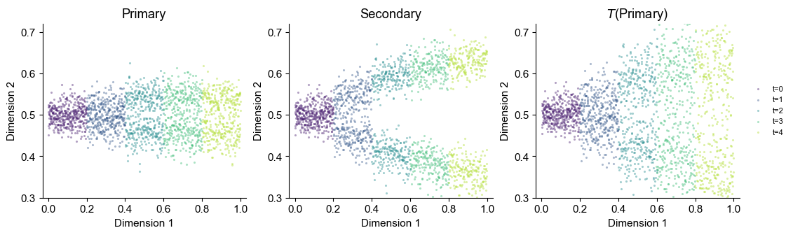
Reproduce the balanced ToySplit branching experiment behind Figure 2b. The primary space contains only weak branch separation, while the paired secondary space amplifies the split. The observations are generated directly from the original seed-42 recipe, assembled as AnnData, and used to refit a time-conditioned map before training the two vector fields. The map is refitted with the original raw-coordinate FiLM architecture, split, loss, optimizer and Sinkhorn checkpoint-selection rule; no legacy checkpoint is loaded.

This notebook compares the balanced RNA-only control with balanced synchronized COATI. The historical unbalanced beta sweep is documented at the end but is not mixed into this BranchSync result.

from pathlib import Path
import sys
import uuid

example_dir = next(parent / "examples" for parent in (Path.cwd(), *Path.cwd().parents)
                   if (parent / "examples" / "synthetic" / "branch_sync.py").is_file())
if str(example_dir) not in sys.path:
    sys.path.insert(0, str(example_dir))

import numpy as np
import pandas as pd
import torch
import matplotlib.pyplot as plt
import coati as ct
from synthetic.branch_sync import (
    TIME_POINTS,
    make_anndata,
    evaluate_map,
    train_historical_map,
    plot_data_and_map,
    plot_branch_comparison,
    branch_diagnostics,
)
from synthetic.gaussian_comparison import make_shared_initial_checkpoint

%matplotlib inline
torch.set_num_threads(1)
plt.rcParams.update({"font.family": "Arial", "font.size": 11})
run_dir = Path("outputs") / ("branch-sync-" + uuid.uuid4().hex[:8])
run_dir.mkdir(parents=True)
print("Result directory:", run_dir)

Result directory: outputs/branch-sync-cfe1d393

Generate the paired snapshots

The spatial coordinate uses five adjacent bins on \([0,1]\). COATI training time is kept on the historical \(0,1,2,3,4\) grid. Each snapshot contains 400 paired cells in the same row order. These spatial bins and model times are distinct quantities.

cells = make_anndata(n_per_time=400, seed=42)
data = ct.TemporalData.from_anndata(
    cells, obsm_key="X_latent", secondary_obsm_key="X_secondary"
)
summary = cells.obs.groupby(["time", "celltype"], observed=True).size().rename("Cells").to_frame()
assert data.times.tolist() == TIME_POINTS.tolist()
assert [len(snapshot) for snapshot in data.primary] == [400] * 5
summary

		Cells
time	celltype
0.0	shared	400
1.0	lower	200
	upper	200
2.0	branch_A	200
	branch_B	200
3.0	branch_A	200
	branch_B	200
4.0	branch_A	200
	branch_B	200

Fit and inspect the cross-modal map

The map follows the original three-layer FiLM architecture with width 64 and a 32-dimensional time embedding. It is trained on raw coordinates with no feature or time standardization. Twenty percent of each stage is withheld; every fifth epoch is ranked by the sum of per-stage validation Sinkhorn divergences.

T, map_report = train_historical_map(cells, run_dir / "map", seed=0)
validation_scores = pd.DataFrame(map_report["stages"]).set_index("time")[
    ["validation_cells", "paired_rmse", "r2", "sinkhorn"]
]
map_scores = evaluate_map(cells, T)
print("Selected map epoch:", map_report["best_epoch"])
display(validation_scores.round(6))
map_scores.round(6)

Selected map epoch: 295

	validation_cells	paired_rmse	r2	sinkhorn
time
0.0	80	0.002397	0.996650	0.000006
1.0	80	0.016145	0.919880	0.000112
2.0	80	0.017249	0.954185	0.000161
3.0	80	0.023427	0.937998	0.000393
4.0	80	0.027798	0.925834	0.000607

	Pairs	RMSE	R2
Time
0.0	400	0.002467	0.996879
1.0	400	0.017010	0.911787
2.0	400	0.015650	0.962201
3.0	400	0.021392	0.947993
4.0	400	0.026780	0.934251

plot_data_and_map(cells, T);

Configure the balanced comparison

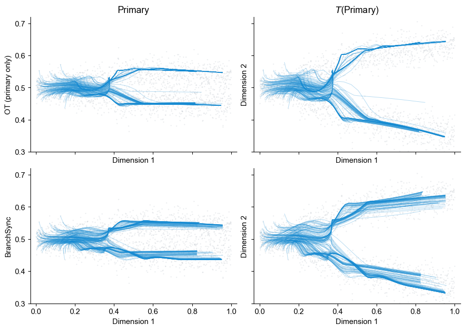
Both vector fields use the Figure 2b architecture and training budget: width 256, two LeakyReLU layers, batch size 128 and 10,000 iterations. The synchronized model uses \(C_y=0.9\) and secondary manifold weight 100; the RNA-only control uses manifold weight 1. Primary matching uses coefficient 10, while BranchSync uses secondary matching coefficient 100. The kinetic-energy weight is 0.1.

adaptive = {
    "adaptive_lambda": True,
    "median_n_sample": 128,
    "floor_n_sample": 128,
    "floor_buffer_std": 1.0,
    "pdf_coefficient_sec": 100.0,
    "lambda_init": 10.0,
    "lambda_min": 1.0,
    "lambda_max": 10.0,
    "eta_lambda": 1.0,
    "lambda_init_pri": 10.0,
    "lambda_init_sec": 100.0,
    "lambda_min_pri": 1.0,
    "lambda_min_sec": 1.0,
    "lambda_max_pri": 10.0,
    "lambda_max_sec": 100.0,
    "eta_lambda_pri": 1.0,
    "eta_lambda_sec": 1.0,
    "dual_warmup": 1000,
    "dual_decay": 1.0,
    "dual_update_freq": 10,
    "dual_ema_alpha": 0.1,
    "lambda_update_mode": "max",
    "eta_neg_scale": 100.0,
}
common = dict(
    balanced=True,
    iterations=10_000,
    batch_size=128,
    hidden_dim=256,
    n_layers=2,
    activation="leaky_relu",
    learning_rate=1e-3,
    energy_weight=.1,
    matching_weight=10.,
    seed=0,
    extra=adaptive,
)
configs = {
    "OT (primary only)": ct.Config(multimodal=False, manifold_weight=1., **common),
    "BranchSync": ct.Config(multimodal=True, secondary_weight=.9,
                            manifold_weight=100., **common),
}
pd.DataFrame({name: {key: cfg.to_dict()[key] for key in
    ["niters", "num_samples", "hidden_dim", "sync_loss", "sync_weight",
     "energy_coefficient", "pdf_coefficient", "density_coefficient"]}
    for name, cfg in configs.items()})

	OT (primary only)	BranchSync
niters	10000	10000
num_samples	128	128
hidden_dim	256	256
sync_loss	False	True
sync_weight	0.0	0.9
energy_coefficient	0.1	0.1
pdf_coefficient	10.0	10.0
density_coefficient	1.0	100.0

Train from the same initialization

The two runs start from one common weight-only checkpoint. The synchronized run receives the frozen fitted map; the control sees only the primary snapshots.

initial = make_shared_initial_checkpoint(
    configs["OT (primary only)"], run_dir / "initial.pt"
)
results = {}
for name, config in configs.items():
    print("Training:", name, flush=True)
    slug = "primary-only" if not config.multimodal else "branch-sync"
    results[name] = ct.fit(
        data,
        config,
        output_dir=run_dir / slug,
        T_model=T if config.multimodal else None,
        warm_start_path=initial,
    )

Training: OT (primary only)

Training: BranchSync

Compare the learned branches

All 400 initial particles are integrated on the historical 0–4 grid. Thin lines show a fixed display subset; the two thick lines summarize the upper and lower distribution halves. The same frozen map is applied to both primary trajectories for a direct secondary-space comparison.

prediction_times = np.linspace(0., 4., 41)
predictions = {
    name: result.predict(times=prediction_times, method="rk4")
    for name, result in results.items()
}
plot_branch_comparison(cells, T, results, predictions);

separation = branch_diagnostics(cells, T, results, predictions)
endpoint = pd.DataFrame({name: result.evaluate() for name, result in results.items()}).T
display(separation.round(6))
endpoint[["endpoint_sinkhorn_after", "kinetic_energy_mean"]].round(6)

	Primary terminal separation	Mapped terminal separation	Secondary endpoint Sinkhorn
Model
OT (primary only)	0.093899	0.267969	0.000615
BranchSync	0.094217	0.269675	0.000302

	endpoint_sinkhorn_after	kinetic_energy_mean
OT (primary only)	0.000419	0.090173
BranchSync	0.000251	0.090611