Gastrulation dynamics and mass

Train a short multimodal, unbalanced COATI model on real mouse gastrulation snapshots, then display E8.5 cell types, instantaneous growth and projected flow on the existing RNA UMAP. Then decompose the change in one cell type over a chosen interval into incoming, outgoing and reweighting.

COATI recommends Scanpy-compatible names; Scanpy itself permits other column names.

Field	Meaning
obs["celltype"]	Supplied categorical cell annotations
obs["time"]	Numeric times in model-training units
obs["barcode"] and obs_names	Matching, globally unique cell identities
obsm["X_umap"]	Existing display coordinates in the same row order

Install with python -m pip install -e '.[notebooks,visualization]'. This notebook uses the prepared gastrulation/rna.h5ad and atac.h5ad from TraInfBench. Source data: Argelaguet and colleagues, GSE205117. Change DATA_DIR to your local folder; cell matrices and model checkpoints are not bundled in COATI.

from pathlib import Path
import os
import uuid
import anndata as ad
import numpy as np
import pandas as pd
import matplotlib.pyplot as plt
import coati as ct
from coati import downstream as ds

%matplotlib inline
plt.rcParams.update({"font.family": "Arial", "font.size": 11})
project_dir = Path.cwd().parent if Path.cwd().name == "notebooks" else Path.cwd()
DATA_DIR = Path(os.environ.get("COATI_GASTRULATION_DATA", project_dir.parent / "TraInfBench/data/processed/gastrulation"))

Load paired biological inputs

The prepared inputs contain 35,503 paired cells, RNA PCA50 and ATAC LSI14. X_latent is already scaled: reuse it without applying normalization again. The four model times are 0, 1, 2 and 2.5 for E7.5, E8.0, E8.5 and E8.75.

Verify barcodes and times before attaching ATAC. Missing source annotations are explicitly marked unknown; labels are not inferred. Preparation copies the input, preserves source columns and reuses the existing UMAP.

rna = ad.read_h5ad(DATA_DIR / "rna.h5ad")
atac = ad.read_h5ad(DATA_DIR / "atac.h5ad")
assert rna.obs_names.is_unique and rna.obs_names.equals(atac.obs_names)
np.testing.assert_array_equal(rna.obs["time_point_processed"], atac.obs["time_point_processed"])
missing_labels = int(rna.obs["celltype"].isna().sum())
cell_types = rna.obs["celltype"].astype(object).fillna("unknown")
cells = ct.prepare_anndata(
    rna, use_rep="X_latent", time_key="time_point_processed", celltype=cell_types,
    secondary=atac.obsm["X_latent"], secondary_key="X_atac", warn=False,
)
assert cells.obs_names.equals(rna.obs_names)
np.testing.assert_array_equal(cells.obsm["X_latent"], rna.obsm["X_latent"])
np.testing.assert_array_equal(cells.obsm["X_umap"], rna.obsm["X_umap"])
print(f"Paired cells: {cells.n_obs:,}; missing annotations marked unknown: {missing_labels:,}")
cells.obs.groupby(["stage", "time"], observed=True).size().rename("Cells").to_frame()

Paired cells: 35,503; missing annotations marked unknown: 3,015

		Cells
stage	time
E7.5	0.0	9018
E8.0	1.0	7796
E8.5	2.0	11470
E8.75	2.5	7219

Train for 1,000 iterations

multimodal=True fits a time-conditioned FiLM map on paired RNA/ATAC before vector-field training. balanced=False enables growth and population-mass change. All four stages are used; this is a dynamics example, not a held-out reconstruction experiment.

The explicit settings below are a short CPU demonstration. The secondary weight is 0.35; population counts are observed sampling counts, not absolute biological population sizes. Changing balanced to True produces a motion-only model.

Set RUN_DIR to an existing fitted result to reuse it; leave it as None to train. The displayed outputs reuse the same 1,000-iteration checkpoint used for this tutorial, without additional fitting.

RUN_DIR = None  # Optional existing COATI result directory.
config = ct.Config(
    multimodal=True, balanced=False, iterations=1000,
    batch_size=128, hidden_dim=128, learning_rate=1e-3,
    secondary_weight=.35, matching_weight=50., energy_weight=1.,
    manifold_weight=.1, sync_density_loss=True, seed=0,
)
if RUN_DIR is None:
    output_dir = Path("outputs") / ("gastrulation-dynamics-" + uuid.uuid4().hex[:8])
    result = ct.train_vector_field(cells, config, output_dir=output_dir)
else:
    result = ct.load_result(RUN_DIR)
    for i, time in enumerate(result.data.times):
        mask = cells.obs["time"].to_numpy() == time
        np.testing.assert_array_equal(result.data.primary[i], cells.obsm["X_latent"][mask])
        np.testing.assert_array_equal(result.data.secondary[i], cells.obsm["X_atac"][mask])
print("Training iterations:", result.metadata["config"]["niters"])
print("Training times:", result.data.times)

Training iterations: 1000
Training times: [0.  1.  2.  2.5]

View one stage on UMAP

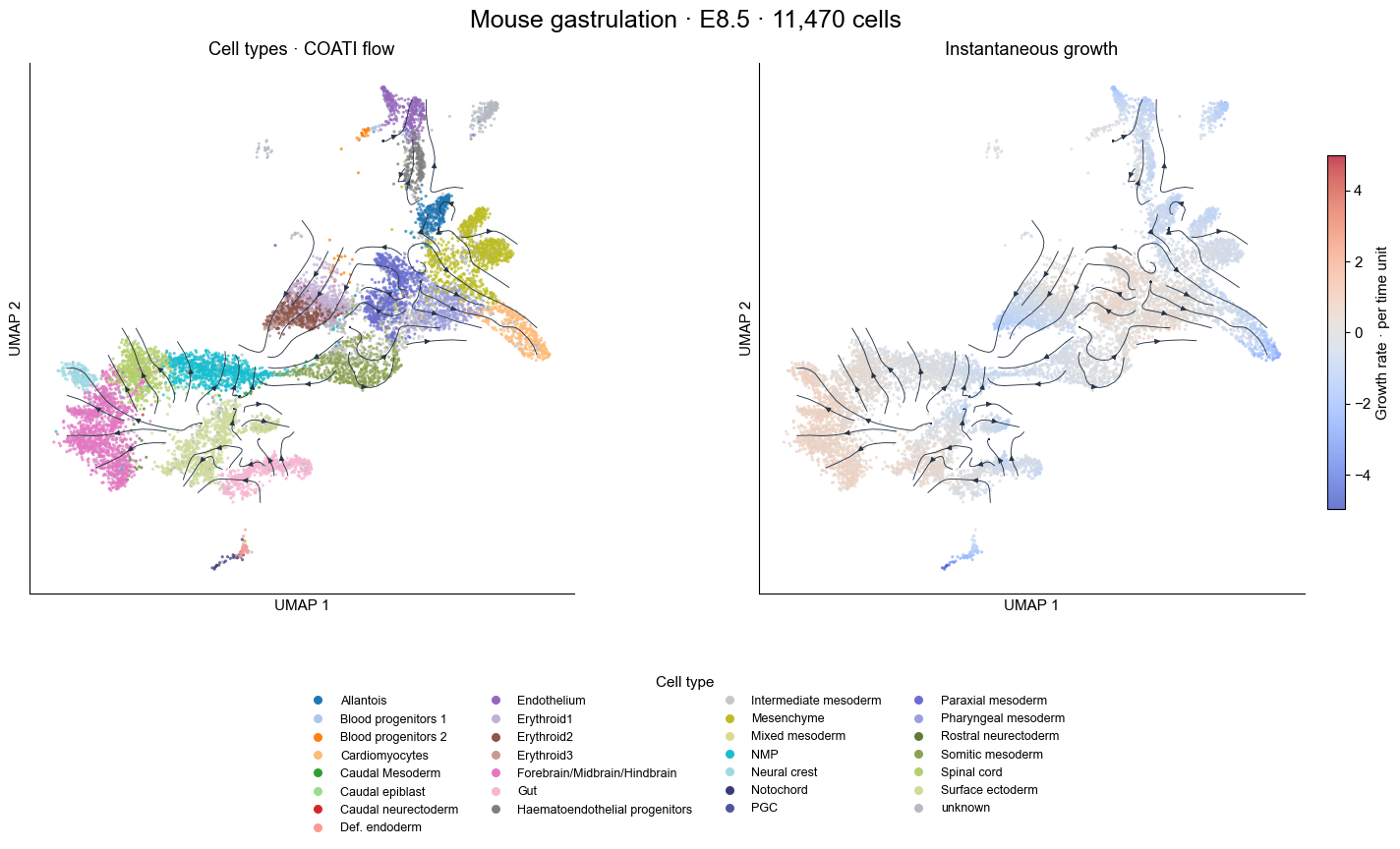
Show all 11,470 E8.5 cells at t = 2. Both panels share coordinates and the same projected COATI velocity field. Cell-type names appear in a common legend to keep the biological plot readable. No toy labels or new UMAP are generated.

The right panel colors instantaneous \(d\log w/dt\), including the saved ODE’s growth multiplier. It is not cumulative weight, cell count or measured proliferation. Streams use a local projection of RNA50 velocities into the existing UMAP; their display resembles RNA velocity, but does not use scVelo’s splicing or transition model.

stage_cells = cells[cells.obs["stage"] == "E8.5"].copy()
names = stage_cells.obs["celltype"].cat.categories
colors = list(plt.get_cmap("tab20").colors) + list(plt.get_cmap("tab20b").colors)
palette = dict(zip(names, colors))
palette["unknown"] = "#b5bac2"
fig, axes = plt.subplots(1, 2, figsize=(15, 9))
result.plot_dynamics(
    stage_cells, axes=axes, labels=False, palette=palette,
    point_size=5, alpha=.75, density=1.3, linewidth=.65, arrow_size=.8, grid_size=60,
)
legend = axes[0].get_legend()
fig.legend(legend.legend_handles, [text.get_text() for text in legend.get_texts()],
           loc="lower center", bbox_to_anchor=(.5, .015), ncol=4,
           frameon=False, fontsize=9, title="Cell type", markerscale=1.3)
legend.remove()
fig.suptitle(f"Mouse gastrulation · E8.5 · {stage_cells.n_obs:,} cells", fontsize=18, y=.96)
axes[0].set_position([.04, .30, .40, .60])
axes[1].set_position([.52, .30, .40, .60])
fig.axes[2].set_position([.935, .36, .012, .47])
plt.show()

Decompose one cell type over a time interval

Change CELLTYPE, START_TIME and END_TIME. This example follows all 9,018 E7.5 particles and examines NMP, E8.0 → E8.5. Keep the full population: selecting only NMP initially would remove incoming trajectories.

At each endpoint, transfer hard cell-type labels from the corresponding observed stage in RNA50 X_latent, not UMAP. n_neighbors=1 matches the paper figure; it can be changed explicitly. All particles remain in the analysis, and endpoint distances and label votes are available in mass.assignments.

Weights are normalized over the full population separately at each time. Incoming uses later weights; outgoing uses earlier weights; reweighting uses the weight difference for particles that remain NMP.

\[\Delta p_{\mathrm{NMP}} = I_{\mathrm{NMP}} - O_{\mathrm{NMP}} + R_{\mathrm{NMP}}.\]

These are relative cell-type proportions, not absolute cell counts or measured causes of proliferation/death. The optional observed marker compares cross-sectional atlas proportions.

CELLTYPE = "NMP"
START_TIME, END_TIME = 1., 2.  # E8.0 -> E8.5 in model time units.

# Integrate the same full source population from E7.5, using a 0.1 solver grid.
trajectory = result.predict_trajectory(times=np.linspace(0., 2.5, 26))
mass = ds.decompose_mass(
    trajectory, cells, celltype=CELLTYPE,
    start_time=START_TIME, end_time=END_TIME,
    use_rep="X_latent", n_neighbors=1,
)
row = mass.summary.loc[CELLTYPE]
assert abs(row["closure_error"]) < 1e-10
print(f"Full source population: {len(mass.assignments):,} particles")
print(f"Predicted {CELLTYPE} proportion: {100 * row.start_proportion:.2f}% -> {100 * row.end_proportion:.2f}%")
pd.DataFrame({"Contribution (percentage points)": 100 * np.array([
    row.incoming, -row.outgoing, row.reweighting, row.net_change,
])}, index=["Incoming", "Outgoing", "Reweighting", "Predicted net change"])

Full source population: 9,018 particles
Predicted NMP proportion: 2.93% -> 9.06%

	Contribution (percentage points)
Incoming	6.688522
Outgoing	-0.265143
Reweighting	-0.297578
Predicted net change	6.125801

STAGE_NAMES = {0.: "E7.5", 1.: "E8.0", 2.: "E8.5", 2.5: "E8.75"}
SHOW_OBSERVED = True
mass.plot(
    show_observed=SHOW_OBSERVED,
    title=f"{CELLTYPE} · {STAGE_NAMES.get(START_TIME, START_TIME)} → {STAGE_NAMES.get(END_TIME, END_TIME)}",
)
plt.show()

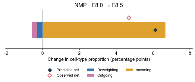
mass.summary contains unsigned incoming/outgoing, signed reweighting and net change in fractions. The figure and table use percentage points, with outgoing shown negatively. mass.transitions groups source and destination labels; mass.assignments retains each particle’s endpoint labels, weights and distances. No paths are dropped by a confidence filter.

This short, one-seed model demonstrates the analysis workflow. The observed atlas change is a reference, not a transition measurement of the same cohort. Interpretation depends on model fit, representation and endpoint label transfer.

Reuse the workflow

python -m examples.gastrulation.dynamics \
    --data-dir /path/to/gastrulation \
    --output outputs/gastrulation-dynamics --iterations 1000 \
    --celltype NMP --start-time 1 --end-time 2

For your own AnnData, reuse the model’s prepared representation and map your metadata columns with ct.prepare_anndata. The decomposition supports balanced predictions with uniform weights; their reweighting component is zero.